Practical implications of free damped vibraton systems.

We all go through the theoretical concepts of vibrations in engineering course work and their understanding is good, but have anyone thought about their practical implications?

From the previous posts on vibration system, I have explained 1 DOF and 2 DOF free damped vibration systems. In this one, I have aimed to explain the practical implications of these free damped vibration systems.

In any vibratory system, theoretically we model the whole system using three basic elements. They are mass which provides inertia to the system, spring which helps in oscillations of the mass and damper which dampens out or reduces the oscillations of the mass. 

Now, practically, based on damping, vibratory systems are categorized into three essential concepts, namely, overdamped, underdamped and critically damped systems. Let’s check examples of each type.

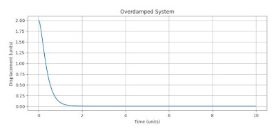
• Automatic door-closer installed in commercial buildings is an example of overdamped system. One can see that once door opens and released it doesn’t swing about the hinge of door but slowly returns to its closed position. Here, the mechanism attached to door on top side acts as damper.

Credits: https://m.indiamart.com/proddetail/aluminum-mosquito-mesh-heavy-door-with-auto-closer-24757497812.html

Figure 1. Overdamped system real life example with corresponding Time-Displacement graph.

• In park, a child’s swing oscillates back and forth, where amplitude decreases slowly over time. This is example of underdamped system where air resistance and swing joints located at top side acts as damper.  

Credits: https://lifestyle.livemint.com/relationships/raising-parents/why-your-kids-need-a-swing-set-111649308702426.html

Figure 2. Underdamped system real life example with corresponding Time-Displacement graph.

• Everyone has seen shock absorber of a bike. Whenever there is bump or pit, we didn’t experience a jerk nor do we oscillate up and down with the bike seat, instead the bike comes to original position without bouncing. This is because of shock absorber located at back side of bike. This is an example of critically damped system.

Credits: https://www.bikedekho.com/tvs/apache-160/images

Figure 3. Critically damped system real life example with corresponding Time-Displacement graph.

Let’s check the applications of damped free vibration in engineering field.

• In electronics industry, design of radio circuits is based on damped vibrations as these circuits work at specific frequencies. These are used for tuning circuits and selecting desired station among many signals.

• It is compulsory to built a earthquake-resistant buildings in earthquake prone areas. This is to prevent collapse of buildings/structures. Damped vibration system plays key role in designing these buildings, as the building itself behaves a damped system, thus resisting/storing and releasing the energies of unexpected shocks.

• In any automobile, the suspension system is designed as a damped system. It is done in order to provide stability and ride comfort. Here, the system is often critically damped.

There is a parameter called damping ratio which is used to determine how fast the oscillation of vibratory system dampens out. Well, what do you think how this is calculated and how this is related to above-mentioned examples?

Equation of motion (translational motion) for 1 DOF discrete vibrational system –

General form of equation of motion is,

ma + cv + kx = 0

The normalized homogenous second order Ordinary Differential Equation for 1 DOF discrete vibrational system is,

a + 2*zeta*v + omega^2*x = 0

Comparing both the equations we get,

zeta = c/(2m)

This zeta is called the damping ratio.

where, m ­= mass of system, 
c = damping coefficient, 
k = stiffness of system, 
a = acceleration, 
v = velocity, 
x = displacement and 
omega = angular eigenfrequency. 

Now, let’s drag the above examples here for explanation using damping ratio.

• Automatic door-closing system is an example of overdamped system, i.e., zeta > 1 or c/(2m) > 1 or, c > 2m. This tells us that the damping coefficient is greater than twice the mass. Thus, the door closes slowly without any oscillations with damping coefficient having upper hand.

• Child’s swing in the park is an example of underdamped system, i.e., zeta < 1 or c/(2m) < 1 or c < 2m. This tells us that the damping coefficient is lesser than twice of mass. Thus, the mass of the system has upper hand and therefore, oscillations are there until the swing stops. 

• Shock absorber of any automobile is an example of critical damped system, i.e., zeta = 1 or c/(2m) = 1 or c = 2m. Thus, the damping coefficient equals twice of mass. This tells us that the damper has sufficient damping coefficient to dampen out oscillations of mass and thus providing comfort ride.

 

Thanks for staying with me till the end. I hope the practical implications is now clear to you guys.

If you want other topic related to mechanical vibrations or from mechanical domain to be explained please tell me in comment section.

Thank you!!

Two-DOF Damped Vibration System.

Hey everyone, welcome back to my blog. This time I am going to tour you through the two degree of freedom free damped vibration system with python implementation. So, lets deep dive into this article.

So, let me ask you a question,

What is 2-DOF damped vibration system?

Any guesses??? 

Nope?? Then, let's check what could be the answer....

A two-degree-of-freedom (2-DOF) free damped vibration system is formed from two masses with two spring and two dampers connected to it. For formulating equations of motion, it involves both the masses. The general representation of a 2-DOF free damped vibration system is as follows,

Consider,

• m1 and  m2 are the masses of first and second body (mass) respectively.
• c1 and c2 are the damping coefficients of the dampers connected to first and second body (mass) respectively.
• k1 and k2 are the stiffness coefficients of the springs connected to first and second body (mass) respectively.
• x1(t) and x2(t) are the displacements of first and second body (mass) respectively as a function of time, t. 
• v1 and v2 are the velocities of first and second body (mass) respectively as a function of time, t.
• a1 and a2 are the accelerations of first and second body (mass) respectively as a function of time, t. 

Figure 1: Spring-mass-damper system of 2 DOF system.

Differential Equations are very much helpful for modelling complex dynamic systems which are time dependent. So, we are going to use this incredible mathematical concept to model our 2-DOF freedom system as follows,

The equations can be written as system of second-order ordinary differential equations (ODEs).

For the first mass (m1),

For the second mass (m2),

Solving the above equations for given initial conditions, which are, x1(0), x2(0), v1(0), v2(0) and parameters m1, m2, k1, k2, c1 and c2 will give us time dependent displacements x1(t) and x2(t), and velocities v1(t) and v2(t) of both masses.

Now, it’s time for some python stuff, so prepare your fingers to hit some buttons!!

# Importing necessary libraries

import numpy as np

from scipy.integrate import odeint

import matplotlib.pyplot as plt

# Defining the system variables

mass1 = 3.0                # Mass of the first mass (kg)

mass2 = 1.0                # Mass of the second mass (kg)

stiffness1 = 30.0          # Spring constant of the first spring (N/m)

stiffness2 = 10.0          # Spring constant of the second spring (N/m)

dampingCoeff1 = 1.5  # Damping coefficient of the first damper (N*s/m)

dampingCoeff2 = 0.5  # Damping coefficient of the second damper (N*s/m)

# Initial conditions

displacement1_0 = 0.5                  # Initial displacement of mass 1 (m)

displacement 2_0 = 0.2                 # Initial displacement of mass 2 (m)

velo1_0 = 0.0                               # Initial velocity of mass 1 (m/s)

velo2_0 = 0.0                               # Initial velocity of mass 2 (m/s)

# Defining function for Ordinary Differential Equations of the 

# 2-DOF system

def TwoDOFsystem(state, time):

    displacement1, displacement2, velo1, velo2 = state

    dx1dt = velo1

    dx2dt = velo2

    dv1dt = (-(stiffness1 + stiffness2) * displacement1 - 

                 (dampingCoeff1 + dampingCoeff2) * velo1 +  

                 stiffness2 * (displacement2 - displacement1) + 

                 dampingCoeff2 * (velo2 - velo1)) / mass1

    dv2dt = (stiffness2 * (displacement1 - displacement2) + 

                 dampingCoeff2 * (velo1 - velo2)) / mass2

   

    return [dx1dt, dx2dt, dv1dt, dv2dt]

# Initialising the time and creating time steps for simulation

time = np.linspace(0, 20, 2000)

 

# Initial state vector

initial_state = [displacement1_0, displacement2_0, velo1_0, velo2_0]

 

# Solve the system of ODEs

solution = odeint(TwoDOFsystem, initial_state, time)

 

# Extract the displacements of mass 1 and mass 2

displacement1 = solution[:, 0]

displacement2 = solution[:, 1]

 

# Plot the displacements

plt.figure(figsize=(10, 6))

plt.plot(time, displacement1, label='Mass 1 Displacement')

plt.plot(time, displacement2, label='Mass 2 Displacement')

plt.xlabel('Time (s)')

plt.ylabel('Displacement (m)')

plt.legend()

plt.grid(True)

plt.title('Two-Degree-of-Freedom Damped Vibration System')

plt.show()

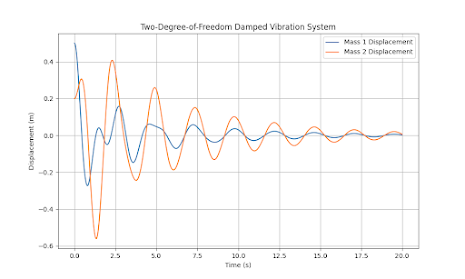
So, let's check how the system behaves from the below plot,

As you can see, the vibrations or displacement diminishes with time. This is because of presence of damper in the system, for each mass.

You can change the values and can play with system accordingly.

Thanks for your attention till the end. If you have any doubts or found some mistake please comment out. I will reach to you. 

If you have any topic related to mechanical field, in mind which needs some python touch please tell me, I will blog it in future.

Thank you all. See you in next blog.

Backyard cultivation of Okra: A health-beneficial vegetable

Hola Amigos!! This time I brought some agriculture related content... 

Everybody reading this article knows about ‘Bhindi’ or in English speaking countries people call it ‘Lady’s Fingers’. But do you know that its actual name is Okra? 

Yes, it sounds somewhat weird. But it's true as Merlin’s Beard.

Okra is a vegetable that is commonly grown in many parts of the world, particularly in Africa, South Asia and southern United States, but not in Germany. Being cultivated in tropical, subtropical and warm temperature regions, okra is used in the cuisines of many countries. Well, it comes in two colours, green and red. 

With a scientific name, Abelmoschus esculentus, the first use of the word okra appeared in 1679 in the Colony of Virginia. Abelmoschus is Neo-Latin from Arabic, while esculentus is Latin which means being fit for human consumption.

Credits - https://unsplash.com/s/photos/okra

Nutritional and Health Benefits - 

• Okra is rich in magnesium, fibre, antioxidants and vitamin C, vitamin K and vitamin A. They support healthy pregnancy, heart health and check blood sugar.
• They contain antioxidants which reduce risk of serious diseases and prevent inflammation. These antioxidants and vitamin C keeps skin healthy and reduces aging.
• Okra contains a thick gel-like substance called mucilage. These binds the cholesterol and thus helps to reduce cholesterol levels, reducing risk of heart disease. 
• Okra is rich in dietary fibre, which can aid in digestion, regulate bowel movements and helps to control appetite and manage weight.  

Refer below for details -  

https://www.healthline.com/nutrition/okra-health-benefits, 

https://www.narayanahealth.org/blog/benefits-of-okra/

Well, coming to day-to-day life, one can grow Okra in their backyard. No, I am not joking.

So, let’s see how is this possible…..

Terrace or backyard gardening is now-a-days very much popular in urban
areas. Generally, steps involved for terrace or backyard gardening are, 

• Suitable containers – Select large containers with depth of 12-18 inches. Check whether the containers have proper drainage system or not, otherwise plants will get damaged if water got logged in container.

• Soil - Use a rich in nutrients soil mix, especially coco peat or organic manure for proper growth of plants.

• Sunlight – These plants need plenty of sunlight so, place them at a location where they will receive at least 5-8 hours of sunlight.

Credits - https://unsplash.com/s/photos/okra

• Planting seeds – One can plant the seed directly to soil or can purchase germinated seeds or seedlings. For seed planting, one should plant them approx. 1 inch deep from soil surface. But one seed per container should be followed.

• Watering – Since, these containers dry out sooner than soil bed, so they need frequent watering to keep plants hydrated. It is better to water plants at root side, in order to avoid growth of fungus at foliage and thus will lead to fungal disease.

• Fertilizing – It is better to use slow-release fertilizer or, a water-soluble fertilizer. If you want you can go organic and can use organic fertilizers like vermicompost. This should be done once plant is grown 5-7 inches and continued through the growing season

• Harvesting – The okra pods are generally ready to harvest in 3 months, and they ae around 2-4 inches long. Harvesting them frequently will promote more pods to develop and grow.   

Credits - https://unsplash.com/s/photos/okra

Thanks for staying with me till the end. 

Please do like subscribe and share.

Breaking down the complexity : Modelling Dynamic Systems with Python implementation.

Hello everyone!! 

I hope everyone reading this is safe and doing well. 

Yes, I know that in blog title agriculture comes first but in this article I have discussed about technology, i.e., Python and how a Mechanical Engineer can use it in Vibration Analysis of any mechancial system. 

So, buckle up your seat belts and get ready for this Python-ic ride!!

Introduction - 

Modelling dynamic systems manually is a tedious task. By the application of Python, a powerful programming language, one can reduce the heavy work and can easily model any dynamic system. This is possible because of python libraries and frameworks designed for scientific computing and simulation.

Described below are the steps and tools required to model a dynamic system using python,

• Select a suitable modelling approach – One can select from differential equations or state space models.

• Choose suitable Python libraries – Python language is rich in libraries which are used for scientific computing and simulation. Some of them are,
• NumPy – It is called numerical python, a collection of numerical computation formulas NumPy.
• SciPy – It is called scientific python SciPy.
• SymPy – It is symbolic python SymPy.
• Matplotlib – This one is used for plotting all kinds of graphs Matplotlib.
• SimPy – This is used for simulation purpose SimPy.
• TensorFlow – This is a collection of a large number of libraries, which is used for machine learning and deep learning tasks TensorFlow.

• Define the Model – Write or derive all the equations necessary to define your dynamic system. These equations can be differential equations or any other mathematical representation. 

• Implementation – Convert your mathematical model to python code for execution. You can do this by creating functions, classes or creating your own libraries.

• Solving the model – Depending upon the method you used for defining your mathematical model, you can solve it using one of the above-mentioned libraries. For example, SciPy’s ‘odeint’ function is commonly used for solving ordinary differential equations.

• Visualization – Matplotlib library is useful for this visualization task. You can create line plots, 2D or 3D plots, or bar graphs etc., according to your need.

 

Now let’s head towards a simple example on modelling dynamic system by python implementation.

 

Problem – Simulation of One dimensional mass-spring-damper system.

A mass-spring-damper system is given with initial conditions and needs to be evaluated for 10 seconds. Since no external disturbances are there so it is a case of free damped vibration. Finite difference method is used for modelling the physics of this problem.

Given, 

mass = 2 kg, 
stiffness = 50.0 N/m, 
damping coefficient = 1.2 Ns/m, 
initial displacement = 2 m 
initial velocity = 0 m/s.

Solution –

The general equation of 1D equation of motion for free damped vibration system (mass-damper-spring system) is given by,

ma + cv + kx = 0,

where, m = mass 

a = acceleration,
c = damping coefficient,
v = velocity,
k = stiffness,
x = displacement.

 

We will use this equation for finding acceleration and then corresponding velocity and displacement.

Let’s jump directly to python implementation. You can use any of the softwares for running the below code, Spyder, Jupyter or Colab.

 

Python code –

 

# Importing necessary libraries

import numpy

import matplotlib.pyplot as plt

 

# System parameters

mass = 2.0                           # Mass (kg)

stiffness = 50.0                    # Spring constant (N/m)

dampCoefficient = 1.2        # Damping coefficient (Ns/m)

 

# Initial conditions

xInitial = 2.0                       # Initial displacement (m)

vInitial = 0.0                       # Initial velocity (m/s)

 

# Simulation parameters

timeStep = 0.01                  # Time step (s)

num_steps = 1000

 

# Defining time, displacement, and velocity variables in the form of

# arrays

time = np.linspace(0, num_steps * timeStep, num_steps + 1)

displacement = np.zeros(num_steps + 1)

velocity = np.zeros(num_steps + 1)

 

# Set initial conditions

displacement[0] = xInitial

velocity[0] = vInitial

 

# Simulate the system using finite differences

for i in range(num_steps):

    # Calculate acceleration (F = ma)

    acceleration = (-stiffness * displacement[i] – dampCoefficient *

    velocity[i]) / mass

 

    # Updating velocity and displacement using Euler's method

    velocity[i + 1] = velocity[i] + acceleration * timeStep

    displacement[i + 1] = displacement[i] + velocity[i + 1] * timeStep

 

# Visualization of model by plotting the graph of displacement vs.

# time

plt.figure(figsize=(10, 4))

plt.plot(time, displacement)

plt.xlabel('Time (s)')

plt.ylabel('Displacement (m)')

plt.title('Simulating motion of 1D Vibration System of mass-spring

damper system)

plt.grid(True)

plt.show()

 

Let’s see how the displacement varies with time,

As we can see from the above graph, 

• Initial displacement is 2 m which is shown in graph.
• With the presence of damper in the system, the displacement decreases with time.
• Negative value of displacement is due to presence of spring, as this spring expands and contracts.

Explanation of the code –

• First, we define the system parameters like mass, spring constant and damping coefficient.
• We set the initial conditions for displacement and velocity.
• Simulation parameters are defined like time step and number of simulation steps.
• We initialise time, displacement and velocity variables.
• We use finite differences method to update the velocity and displacement at each time step based on equation of motion.

So, thank you everyone for staying with me till the end. I hope this article has given you valuable insights on how we can use python for solving complex problems.

Please like and comment about this article and if you want any other type of modelling, you can write it on comment section. Also, please share this to your connections.